
When we count points of two data sets per cell, we can compare their densities. By generating Chi expectation surfaces, we can compare the actual densities with the expected densities. Coming back to our geographic names with “wald” in Switzerland, we could compare whether these names are over- or underrepresented compared to all geographic names.
For better understanding, QGIS commands are marked in bold italics.
We start with a single grid and two layers containing counts per grid cell. One layer should contain the expected resp. underlying population, in our case the counts of all the geographical names per grid cell; the other layer contains the feature we are interested in comparing to the underlying population e.g., the geographical names containing “wald”. If you did part II of the point data tutorial, you will have to create a second layer with the counts of all the geographical names. Make sure to use the same grid for the counting. You don’t need to do any coloring yet.
1. Filter out zero counts cells
For the calculation of the Chi value, we only choose grid cells whose count is bigger than 0, otherwise the formula does not work (↯ zero in the denominator ↯). To filter the values, we open the attribute table of each layer with counts (right click on the layer –> Open Attribute Table). We click on the funnel symbol and filter the column of the counts according to Greater than (>) 0:
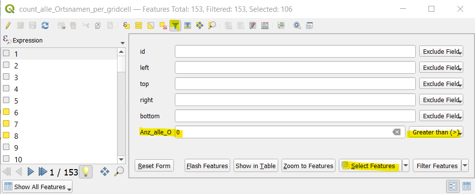
We then click on Select Features and then save the layer by right-clicking on it Export –> Save Selected Features As… We do the same for the other layer.
2. Join the counts into one layer
To calculate the Chi value, we need the counts of both layers in the same attribute table. This means we have to do a join from the “wald” layer to one with all the geographical names. We right click on the layer with the “wald” counts and we choose Properties. In the navigation with the symbols on the left side, we choose Joins. We click on the green plus icon (+) to add a new join. In the newly opened window, we choose the following parameters:
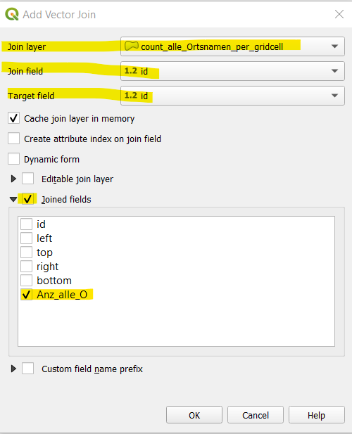
Join Layer: Layer with all the geographical names.
Join und Target field: We choose the id in both layers to join on.
Joined fields: The field we want to add from the layer with all the geographical names to the layer with only the “wald” names.
If the ids match, the layer with the “wald” names gets an entry (with the counts from all the geographical names) in the newly added column for the respective grid cell/row.
We click OK, then Apply and again OK. The join is now listed in the Joins section of Properties.
3. Normalization
Since the two distributions have a different number of features, we have to normalize the formula for the Chi value. To find out how much features there are we click on Vector –> Analysis Tools –> Basic Statistics for Fields. In the newly opened window, we choose the corresponding layer as Input Layer and the Field to calculate statistics on:
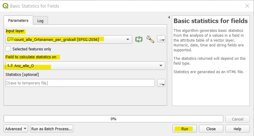
Then we click on Run. The output is a Log file where we are only interested in the ‘SUM’: … Write down this number, then do the same with the other layer.

4. Calculate the Chi Value
To calculate the Chi value, we open the attribute table of the layer with the “wald” names where both of the counts are stored (right click on the layer –> Open Attribute Table). Click on Open Field Calculator (see icon on the right side of this paragraph).
In the field calculator, we start by ticking the box Create a new field. We give it a name (Output field name) e.g., Chi, and choose as type (Output field type) 1.2 Decimal number (real).
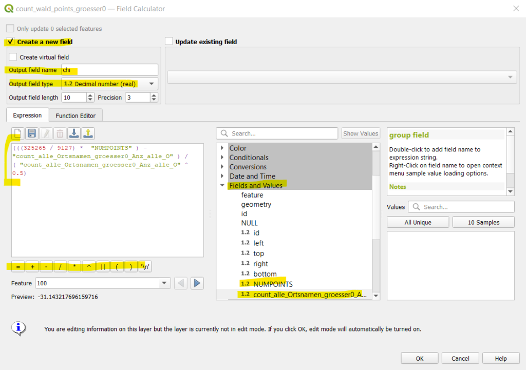
In the middle part, click on Fields and Values to choose the column names from your attribute table.
The formula of the Chi value is:
Chi = (observed frequency – expected frequency ) / √ expected frequency
We will add the sums we just retrieved to normalize the formula as a factor: The number of all the geographical names divided by the number of the “wald” names. In my case it is:
(((258064 / 9127) * Anz_Wald_Ortsnamen) – Anz_alle_Ortsnamen) / √ Anz_alle_Ortsnamen
We enter this formula in the field on the left side. You can use the mathematical operators just below the field or type them and the column names from the Fields and Values in the middle. If the formula is correctly written, you should see a number below the field where it says Preview. Click on OK. In the attribute table you should now see the new column with the Chi values. Save the changes by clicking on the icon with the disk and the red pen.
5. Color the grid cells according to the Chi Value
A negative Chi value means that names with “wald” are underrepresented in this grid cell compared to all the geographical names, while a positive value means an over-representation. We can highlight this difference with a diverging color scheme. We right click on the layer with the Chi value, then we choose Properties –> Symbology.
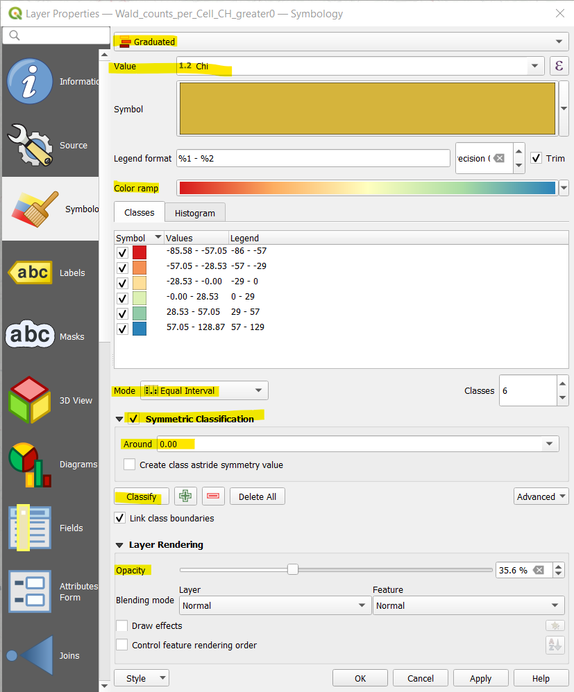
Choose a Graduated color scheme.
Value: Choose the Chi value.
Color Ramp: By clicking on the down arrow, you get a list of possible color ramps or you can even create your own. Further, you can invert any ramp. Since the Chi values are negative and positive, a diverging color scheme makes sense e.g., Spectral. If you want 0 to be in the middle of the color scheme, you can tick the box Symmetric Classification and add 0 in the field Around. You might also want to reduce the Opacity to around 40%. Click on Apply, if you are happy with the map, click on OK, otherwise adapt the symbology.