
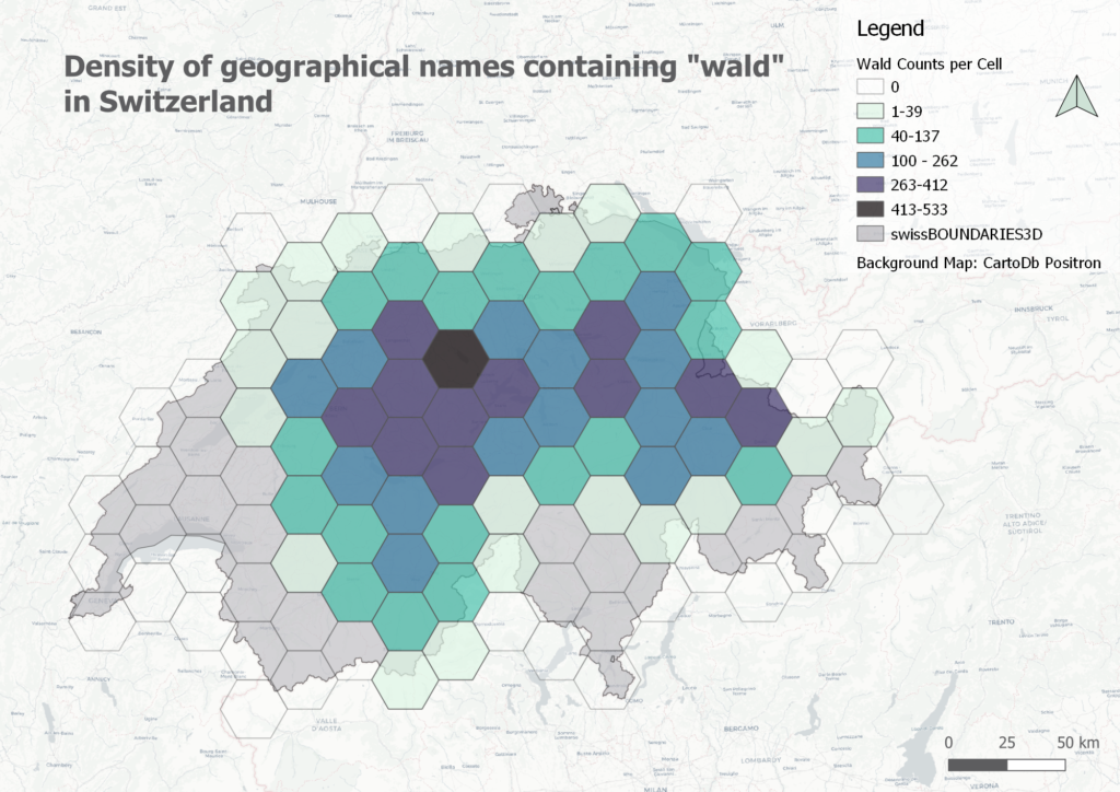
This is part II of the point data tutorial for QGIS. It teaches you how to create a grid and then count the points per grid cell. You can use this hexagonal binning to visualize the density e.g., of geographical names containing “wald” in Switzerland.
For better understanding, QGIS commands are marked in bold italics.
We start with a data set of points that covers the whole of Switzerland e.g., all the geographical names containing “wald” (forest in english).
1. Create a grid
We create a spatial grid with cells of equal area to be able to compare the data points. For that we go to the main navigation and click on Vector –> Research Tools –> Create Grid.
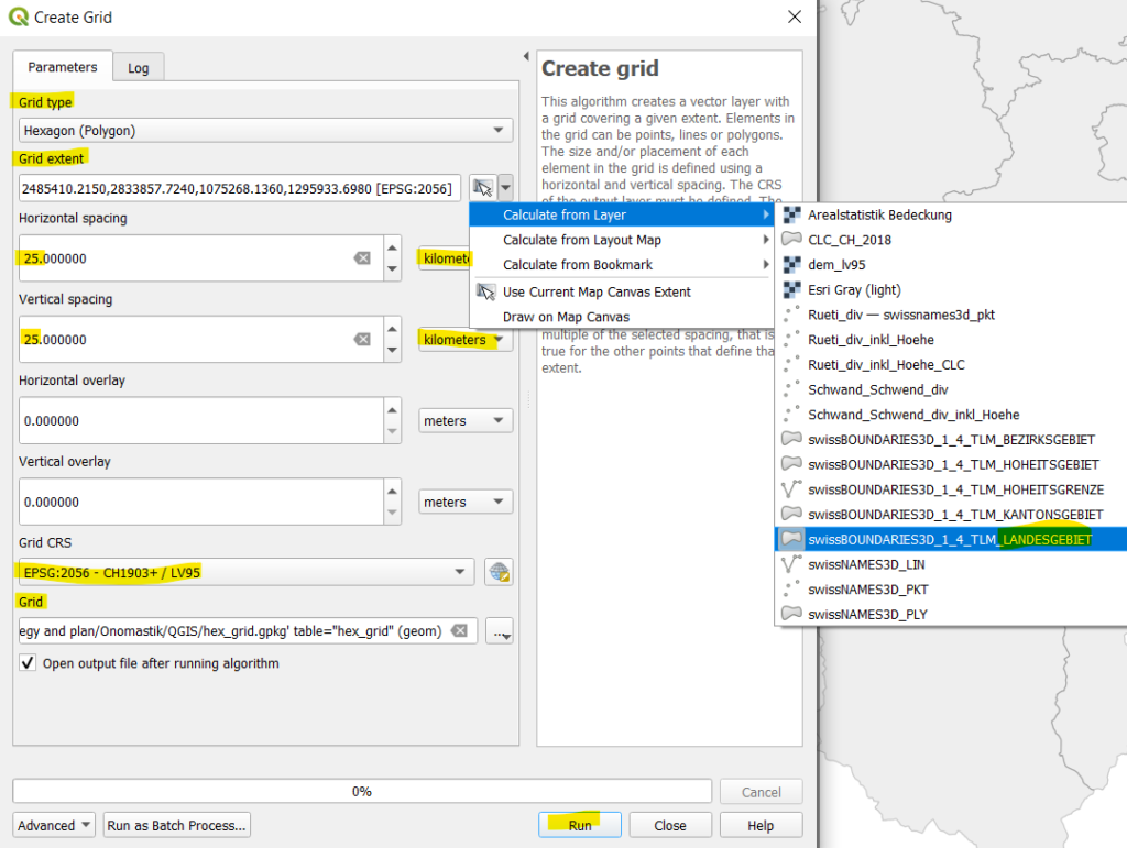
In the window that opens, there are different grid types to choose from. We go for a Hexagon (Polygon). The grid should extend over the entire area of Switzerland. We can tell QGIS to use the extent of another layer, in our case the area of Switzerland (swissBOUNDARIES3D … LANDESGEBIET). The spacing of the grid depends on the area we want to cover. For our study, we will use 25 x 25 km. Make sure to change the unit from meters to kilometers. If you have a smaller study area, reduce the spacing. We further choose the coordinate system (CRS) for the grid. We go for EPSG: 2056 (CH1903+/LV95) in accordance with the coordinate system of our other data. Finally, we set a file name and path to save the grid as a file (click on the three dots …). After you click on Run, a rectangular grid of hexagons is created covering Switzerland.
We do not care about the color of the hexagons now as we will color the grid cells according to the number of points they contain in the next step.
2. Reduce the grid to the outline of Switzerland
Since our grid is rectangular, it now covers much more than just the area of Switzerland. We can get rid of the hexagons entirely outside of Switzerland by select only the grid cells that are within the area of Switzerland.
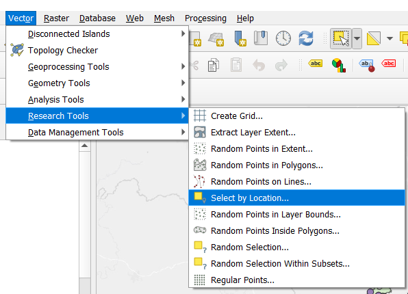
In the main navigation, we click on Vector –> Research Tools –> Select by Location:
In the window that opens, we choose the following parameters:
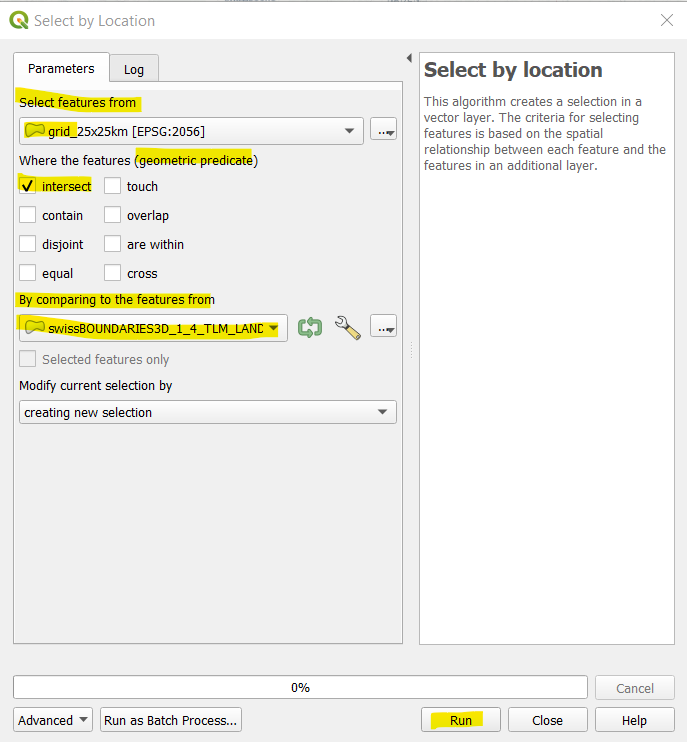
Select features from: The layer with the grid cells and the counts of the “wald” names.
Where the features (geometric predicate): intersect
By comparing to the features from: The layer with the area from Switzerland.
Then click on Run and Close. You see that the grid cells intersecting with the area of Switzerland are now colored in yellow. With a right click on the layer, Export, we Save Selected Features As new a shapefile.
3. Count the points per grid cell
To count the points per hexagon/grid cell, we go to the main navigation and click on Vector –> Analysis Tools –> Count Points in Polygons. In the window that opens you choose the following parameters:
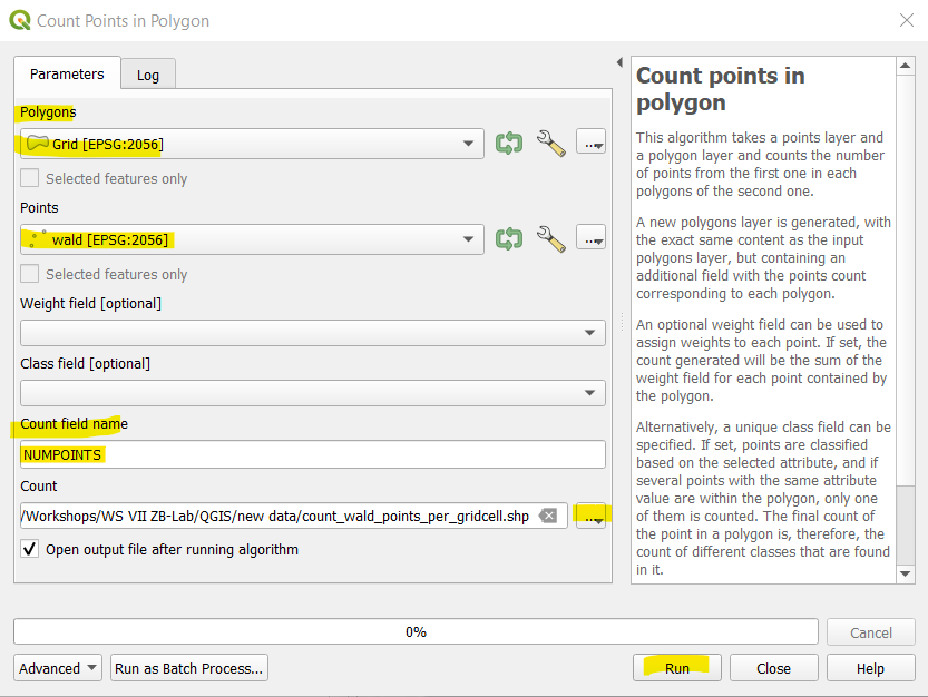
Polygons: Choose your adapted grid.
Points: Choose the layer with the geographical names you want to count (in our case the “wald” layer).
Count field name: This is the new column that is being added to your attribute table and where the counts of the points are stored. Give it a meaningful name. You then save the new layer (…) as file (shp) and click on Run.
The newly created layer looks the same as the grid you created in the step before, but in its attribute table the counts of the geographical names with “wald” are now contained. We now color each grid cell according to its number of points.
4. Color each grid cell according to an attribute
We right click on the newly created layer, choose Properties –> Symbology.
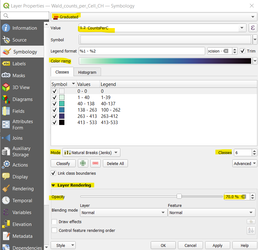
Choose a Graduated color scheme.
Value: Choose the variable according to which you want to color the cell.
Color Ramp: By clicking on the down arrow, you get a list of possible color ramps or you can even create your own. Further, you can invert any ramp e.g., if you want light colors for low and dark for high numbers.
Mode and Classes: You can choose how the counts are split into different classes and how many classes you want to display. The mode and number of classes shown are just an example. Once you are finished, click on Classify and the different classes are created. If you want to adapt the mode or the classes, you have to click on Classify again.
To prevent the hexagons from covering Switzerland, we reduce the opacity under Layer Rendering at the bottom of the window (click on the right arrow), to e.g. 80% (depending on the color gradient you have selected, you may need more or less). Click on Apply and check your map. If you are happy, press OK, otherwise adjust.
Hint: If you want to compare two values, it makes sense to use the same classes (the same breaks). The classes including the colors can be saved (Style –> Save Style) and imported to another value (Style –> Load Style).
Hint 2: Beautiful color gradients are available from ColorBrewer. Here you can set, among other things, that colors should be selected in such a way that also colorblind people can distinguish them. The ColorBrewer color gradients are already stored in QGIS. You can access them by clicking on the down arrow at the Color Ramp –> Create New Color Ramp. Then select as ramp type: Catalog: ColorBrewer. Click OK and all gradients (scheme) will appear for selection.