
You have imported point data into QGIS and want to analyse it further. This short tutorial shows you step by step how you can filter your dataset based on an attribute or on the spatial location. Part II teaches you how to create a grid to calculate a density surface, that is to count the points per grid cell.
Please note: For better understanding, the QGIS commands are marked in bold italics.
1. Set up and Data
In this tutorial, we need a QGIS project like described in this blog post (steps 1 to 5). For step 6, the data, we work with the point data set of swissNames3D, a large collection of Swiss geographic names published by the Federal office of Topography swisstopo. You download the shp file and then you add the swissNAMES3D_PKT.shp as vector layer to your project (Layer –> Add Layer –> Add Vector Layer …). We further use the Swiss boundaries data set (the layer with the different cantons, swissBOUNDARIES3D_1_4_TLM_KANTONSGEBIET.shp, and the layer containing Switzerland, swissBOUNDARIES3D_1_4_TLM_LANDESGEBIET.shp), published by swisstopo as well. They can be added the same way as the swissNAMES3D_PKT layer.
Hint: The order in which the layer appear in the Layers window matters. Imagine a stack, where the layer on top is also on top in the map window. So make sure your background map is at the bottom, otherwise it hides all the other layers.
If you already have your sample of point data and are just interested in the grid, then you can skip the following steps and go directly to part II.
2. Filter the point data
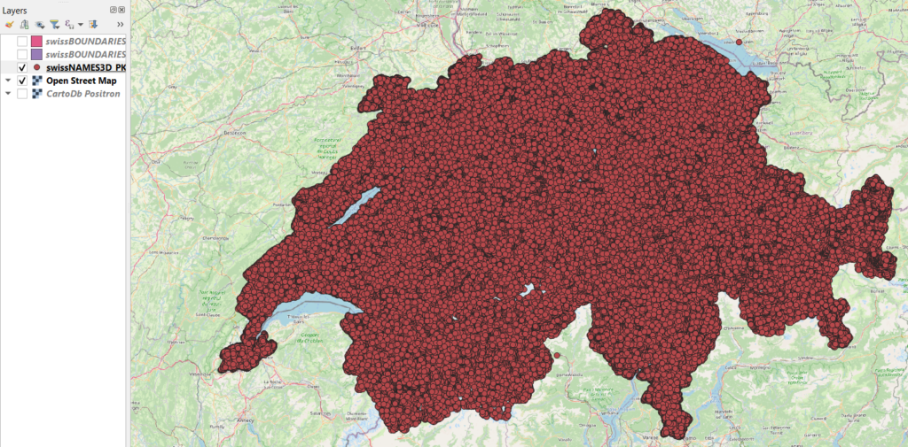
Right now, the swissNames3D_PKT layer has almost 330’000 points. You see them when right clicking on the layer, then choose Open Attribute Table. When displaying the layer, the points cover the entire area of Switzerland. However, we only want a subset of these points which we can create by filtering according to attribute or by spatially intersecting the points with a polygon e.g., a certain canton. We will do both:
a) according to an attribute
Let’s say we are interested in all the geographic names containing the word “wald” (“forest” in English). To filter these names out, we open the attribute table by right clicking on the layer, then Open Attribute Table.
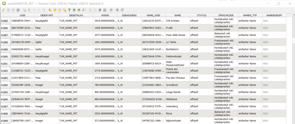
You can imagine the attribute as an excel table containing all your data. To filter the data, we click on the funnel symbol in the middle of the navigation bar (highlighted in yellow in the screenshot below) and we enter “wald” in the field NAME. Then we click on Select Features.
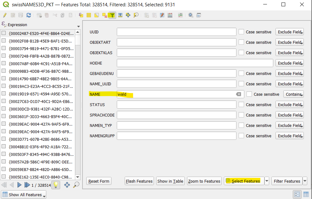
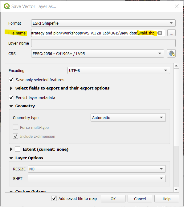
QGIS then filters the data and tells us in the header how many features have been found and selected. To save them in a new layer, we go back to the map (just close the attribute table or minimize it). All the geographic names containing “wald” are now colored yellow. We right click on the layer swissNames3D_PKT, choose Export, then Save Selected Features As… A new window opens, where we click on the three dots … and choose the path where we want to save the features, enter a file name and click on OK.
b) based on its spatial location
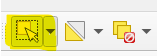
If we only want the geographical names containing “wald” in a certain canton, we have to select the corresponding canton. We make sure the layer with the cantons is displayed on the map and selected (just click once on it in the Layers window). Let’s say we only want the names containing “wald” in Grisons. We can either choose Grisons by attribute as we did in the step before (2a) or go for Select Features by Area or Single Click (click on that symbol with the yellow square and the white arrow). We do the latter. Then you can directly click on the canton to select it. After the selection, the canton should be colored in yellow.
To select the “wald” names in Grisons, you go to the main navigation and choose: Vector –> Research Tools –> Select by Location:
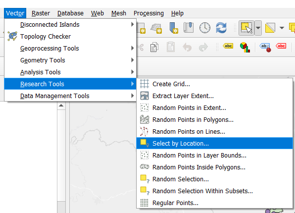
In the new window that opens, you choose the “wald” layer to Select features from. The geometric predicate is are within. In the field By comparing the features from, you choose the swissBoundaries3D_14_TLM_KANTONSGEBIET layer with the cantons, additionally you tick the box Selected features only. Then click on Run. Now, all the “wald” names in Grisons are chosen. We still have to save them by right clicking on the “wald” layer and choosing Save selected features as… as we did before.

Hint: Since we are done with selecting and filtering data, we can deselect everything by clicking on the symbol on the right (Deselect Features from All Layers).
Now, we are ready for part II: create a grid and count the points per grid cell …